

A guide to optimizing Transformer-based models for faster inference


Have you ever suffered from high inference time when working with Transformers? In this blog post, we will show you how to optimize and deploy your model to improve speed up to x10!
If you have been keeping up with the fast-moving world of AI, you surely know that in recent years Transformer models have taken over the state-of-the-art in many vital tasks on NLP, Computer Vision, time series analysis, and much more.
Although ubiquitous, many of these models are very big and slow at inference time, requiring billions of operations to process inputs. Ultimately, this affects user experience and increases infrastructure costs as heaps of memory and computing power are needed to run these models. Even our planet is affected by this, as more computing power demands more energy, which could translate to more pollution.
One solution for accelerating these models can be buying more powerful hardware. However, this isn’t a very scalable solution. Also, it may be the case that we can’t just use bigger hardware as we may want to run these models on the edge: mobile phones, security cameras, vacuum cleaners, or self-driving vehicles. By nature, these embedded devices are resource-constrained, with limited memory, computing power, and battery life. So, how can we make the most out of our hardware, whether a mobile phone or a huge data center? How can we fit our model in less memory, maintaining accuracy? And how can we make it faster or even run in real time?

The answer to these questions is optimization. This blog post presents a step-by-step guide with overviews of various techniques, plus a notebook hosted on Google Colab so you can easily reproduce it on your own!

Our code is available here.
You can apply many optimization techniques to make your models much more efficient: graph optimization, downcasting and quantization, using specialized runtimes, and more. Unfortunately, we couldn’t find many comprehensive guides on how to apply these techniques to Transformer models.
We take a fine-tuned version of the well-known BERT model architecture as a case study. You will see how to perform model optimization by loading the transformer model, pruning the model with sparsity and block movement, converting the model to ONNX, and applying graph optimization and downcasting. Moreover, we will show you how to deploy your optimized model on an inference server.
Try it out
We prepared and included the following live frontend on a 🤗 Hugging Face space so you can test and compare the baseline model, which is a large BERT fine-tuned on the squadv2 dataset, with an already available pruned version of this baseline, and finally, our ‘pruned + optimized’ version!
In the interactive demo below, you will see three fields:
- the
Modelfield, where you can select any of the three models mentioned before (by default, our optimized model). - the
Textfield, where you should provide context about a topic. - the
Questionfield, where you can ask the AI about something in the text.
You can also try the demo here.
Question Answering (QA) models solve a very simple task: retrieve the answer to questions about a given text.
Let’s take the following text as an example:
“The first little pig was very lazy. He didn't want to work at all and he built his house out of straw. The second little pig worked a little bit harder but he was somewhat lazy too and he built his house out of sticks. Then, they sang and danced and played together the rest of the day.”
Question: “Who worked a little bit harder?”
Expected answer: “The second little pig.”
You can try this example on our live demo and see if the model gives the right answer!
Note that state-of-the-art QA models can only correctly answer questions that can be answered as a specific portion of the input text. For example, if the question was “Which pigs are lazy?” the correct answer should be something like “the first little pig and the second little pig” or “the first and second little pigs”. However, a QA model won’t give any of these answers as they do not appear as such in the text.
If you select the prunned version of the model or our prunned + optimized version you should see shorter inference times. Also, you might see differences in the answers given by each model. For the example text provided above, try asking, “What did the pigs do after building their house?”.
The optimization journey
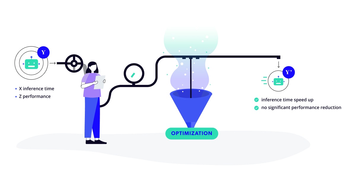
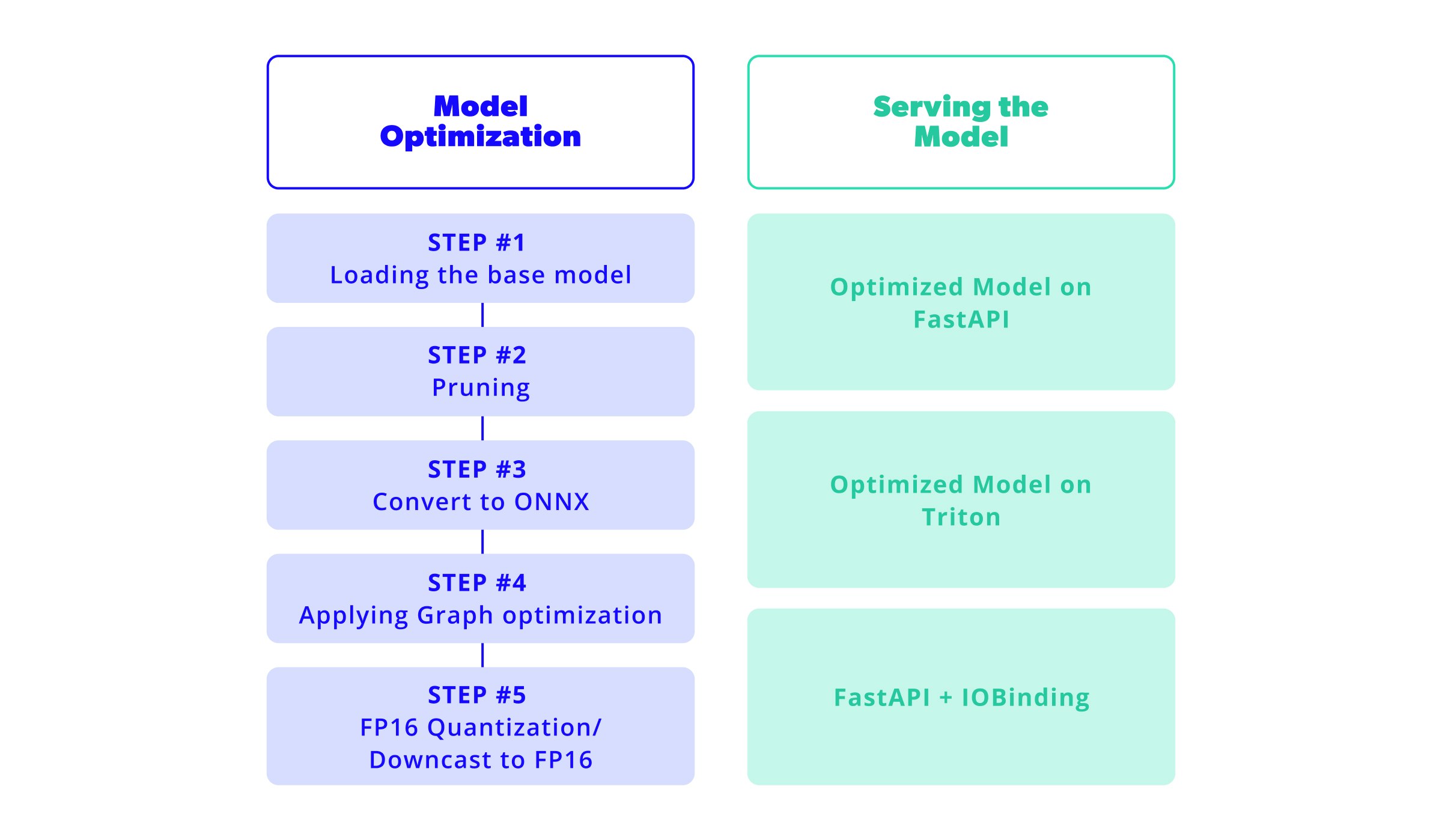
Now let's walk together through the optimization path to get to a blazing fast model! We need to take care of two main tasks: optimizing the model and serving the model. The following diagram gives a broad overview of the steps needed to walk this road. And we know there are a few, but a journey that only takes two steps to complete isn’t really that memorable, is it?

1. Model Optimization
Step #1: Loading the base model
Load a Pre-Trained Model
Thanks to 🤗 Hugging Face’s model zoo and the transformers library, we can load numerous pre-trained models with just a few lines of code!
Check out the from_pretrained() function on the transformers documentation!
As a starting point, we will need to select which model to use. In our case, we will be working with madlag/bert-large-uncased-whole-word-masking-finetuned-squadv2, a BERT Large model fine-tuned on the dataset squad_v2. The SQuAD 2.0 dataset combines 100,000 questions in SQuAD 1.1 with over 50,000 unanswerable questions to look similar to answerable ones. This dataset and the trained model aim to resolve the problem of question answering while abstaining from answering questions that cannot be answered.
We can load this model in Python with the help of 🤗 Hugging Face’s transformers library by using the AutoModelForQuestionAnswering and AutoTokenizer classes in the following way:
This code will load the tokenizer and model and save this last one inside models/bert.
This model will be our starting point of comparison. We will check different metrics to evaluate how well we are optimizing in each step.
We will take a special look at the following:
- Model size: the size of the exported model file. It is important as it will impact how much space the model will take on the disk and loaded in the GPU/RAM.
- Model performance: how well it performs after each optimization with respect to the F1 score over the SQUADv2 validation set. Some steps of the optimization may affect the performance as they change the structure of the network.
- Model throughput: this is the metric we want to improve in each step (for the context of this blog post) and we will measure it by looking at the model’s inference speed. To do this, we will use Google Colab in GPU mode. In our case the assigned GPU was an NVIDIA Tesla T4, and we will test it with the maximum sequence supported by the model (512 characters).
To measure inference speed, we will be using the following function:
You can find the definition of the benchmark function inside the Google Colab.
The metrics for the baseline model are:
| Model size | 1275M |
| Model performance (Best F1) | 86.08% |
| Model throughput (Tesla T4) | 140.529 ms |
Step #2: Pruning
Reduce model size via Pruning
In this step, we will prune the model. Pruning consists of various techniques to reduce the size of the model by modifying the architecture.
It works by removing weights from the model architecture, which removes connections between nodes in the graph. This directly reduces model size and helps reduce the necessary calculations for inference with a downside of losing performance as the model is less complex.
There are different approaches to pruning a neural network. We will be using Neural Networks Block Movement Pruning which uses a technique called sparsity. This work is backed by 🤗 Hugging Face, thanks to the library nn_pruning. You can learn more about how this works internally on the blogs [1, 2] posted by François Lagunas.
As a first step in optimizing the model, we will use pruning. Thankfully a pruned version of our base model already exists for us to use, post-training tuning included (sometimes called fine-pruning or fine-tuning a pruned model). This step is advised as the model changes, and performance will be affected. When we train the new model, we adapt the new weights to prevent losing performance.
This pruned model is available in the 🤗 Hugging Face model zoo. If you want to prune a custom model, you can follow this notebook tutorial on how to do so in a few simple steps.
Similar to the previous step, let’s load this pruned model:
This code will load the tokenizer and model and save it to models/bert_pruned.
Let’s compare this model to the baseline one. We can see an improvement in reducing the size by 14.90% and increasing the throughput by x1.55 while the performance decreased by 3.41 points.
| Model size | 1085M |
| Model performance (Best F1) | 82.67% |
| Model throughput (Tesla T4) | 90.801 ms |
Step #3: Convert to ONNX
The ONNX format
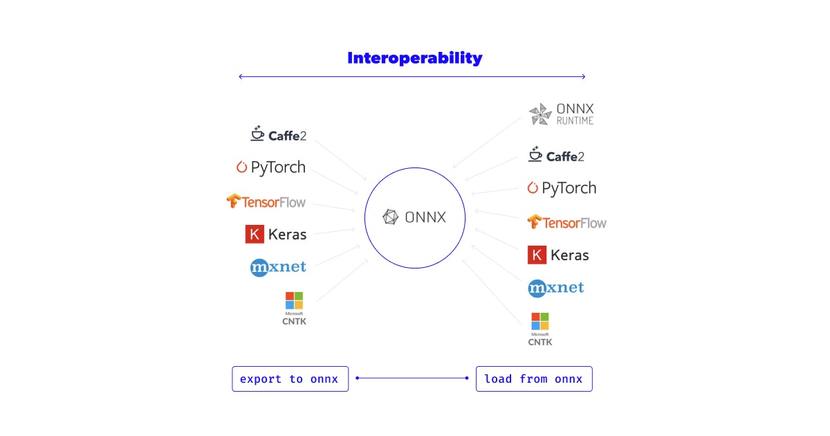
ONNX (Open Neural Network Exchange) is an open format to represent machine learning models by defining a common set of operators for the model architectures.
Many frameworks for training models (PyTorch, TensorFlow, Caffe2, etc.) allow you to export their models to ONNX and also import models in ONNX format. This enables you to move models from one framework to another.
Training frameworks, like the ones mentioned above, are usually huge libraries requiring significant space and time to install and run. An advantage of converting our models to ONNX is that we can run them in small footprint libraries such as onnxruntime, giving us more space and a speed boost in our production environment.

The next step is to convert our model to ONNX. To do this, we can take advantage of the optimum library from 🤗 Hugging Face, which helps us make our models more efficient in training and inference. In our case, we will take advantage of the implementations for ORT (ONNX Runtime).
Optimum provides us the ability to convert 🤗 Hugging Face models to ORT. In this case, we will use ORTModelForQuestionAnswering but keep in mind that there are options for the model of your choice.
This class takes a 🤗 Hugging Face model and returns the ORT version of it. Let’s use it to transform our pruned model to ORT.
This code will load the tokenizer and model and save it to models/bert_onnx_pruned/model.onnx.
In this step, the model size and the model performance stay still, as we do not generate a change in the architecture. However, thanks to the new execution environment, we can see an improvement in the model throughput of x1.18 compared to the previous step and x1.83 compared to the baseline model.
| Model size | 1085M |
| Model performance (Best F1) | 82.67% |
| Model throughput (Tesla T4) | 76.723 ms |
Step #4: Applying Graph optimization
Graph Optimization
Converting our model to ONNX means having a new set of tools at our disposal to optimize the models. An ONNX graph can be optimized through different methods.
One of them is node fusion, which consists of combining, when possible, multiple nodes of the graph into a single one and by doing so making the whole graph smaller.
Another method is constant folding, which works in the same way as in compilers. It pre-computes calculations that can be done before running the inference on the model. This removes the need to compute them on inference.
Redundant node elimination is another technique for removing nodes that do not affect the inference of a model, such as identity nodes, dropout nodes, etc. Many more optimizations can be done in a graph; here is the full documentation on the implemented optimizations on ORT.
In this step, we will optimize the ONNX graph with the help of ORT, which provides a set of tools for this purpose. In this case, we will be using the default optimization level for BERT-like models, which is currently set to only basic optimizations by default.
This will enable constant folding, redundant node elimination and node fusion. To do this, we only need to write the following code:
This code will optimize the model using ORT and save it to models/bert_onnx_pruned/optimized.onnx.
In this step, the model’s size and performance also stay the same as the basic optimizations do not interfere with the result of the model itself. However, they impact the throughput due to reducing the number of calculations taking place. We can see an improvement of x1.04 compared to the previous step and x1.9 compared to the baseline model.
| Model size | 1085M |
| Model performance (Best F1) | 82.67% |
| Model throughput (Tesla T4) | 73.859 ms |
Step #5: Downcast to FP16
Downcasting
Downcasting a neural network involves changing the precision of the weights from 32-bit (FP32) to 16-bit floating point (half-precision floating-point format or FP16).
This has different effects on the model itself. As it stores numbers that take up fewer bits, the model reduces its size (hopefully, as we are going from 32 to 16 bits, it will halve its size).
At the same time, we are forcing the model to do operations with less information, as it was trained with 32 bits. When the model does the inference with 16 bits, it will be less precise. This might affect the performance of the model.
In this step, we will reduce the precision of the model from 32 bits to 16. Thankfully onnxruntime has a utility to change our model precision to FP16. The model we have already loaded from the previous step has a method called convert_float_to_float16, which directly does what we need! We will be using deepcopy to create a copy of the model object to ensure we do not modify the state of the previous model.
This code will load the tokenizer and model and save it to models/bert_onnx_pruned/optimized_fp16.onnx.
After this step, the size of the model was reduced by 49.03% compared to the previous one. This is almost half the size of the model. When compared to the baseline model, it decreased by 56.63%.
Surprisingly, the performance was affected positively, increasing by 0.01%. This means that using the half-precision model, in this case, is better than using the FP32 one.
Finally, we see a huge change in the throughput metric, improving x4.06 compared to the previous step. If we compare this against the baseline model, it is x7.73 faster.
| Model size | 553M |
| Model performance (Best F1) | 82.68% |
| Model throughput (Tesla T4) | 18.184 ms |
When we applied Downcasting, we converted the weights and biases of our model from a FP32 representation to a FP16 representation. An additional optimization step would be to apply Quantization, which takes it one step further and converts the weights and biases of our model to an 8-bit integer (INT8) representation. This representation takes four times less storage space, making your model even smaller! Also, operating with INT8 is usually faster and more portable, as almost every device supports integer operations, and not all devices support floating-point operations. We didn’t apply quantization during this model optimization concretely. However, it is a good technique to consider if trying to optimize arithmetic processing mainly on the CPU or reduce the model’s size.
Intermediate summary
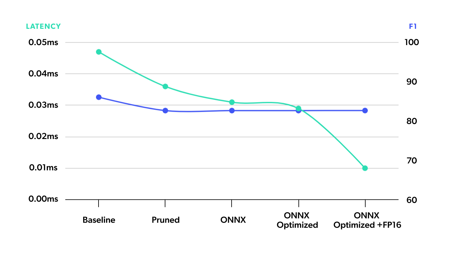
As the final result, we have a model that is almost half the size, loses only 3.24 performance points, and runs x7.73 times faster when compared to the original one. We can see a comparison of each step in the graph below, where we seek to have a high number in F1 and a low number in latency.

2. Serving
Now we have a super-fast and lightweight version of our model, so what’s next? Well, you will surely want to make your model accessible to users, so it’s time to take it to production! This section shows you how to easily and efficiently serve your model while testing several strategies. You can also check this work done by Michaël Benesty on a different BERT model.
If you have ever tried to deploy a model, you have probably heard of FastAPI. FastAPI is a well-known open-source framework for developing Restful APIs in Python, developed by Sebastián Ramirez. It is user-friendly, performant, and can help you get your model up in a matter of minutes. Without a doubt, it is one of the first choices for every ML/DS engineer to get the first version of their model up and running!
We benchmark the different deployment strategies with different sequence lengths on the input. For each sequence length, we send 50 sequential, random requests and report the server's mean and standard deviation response time.
Here is the benchmark of the base model deployed on FastAPI.
| Sequence Length | Mean Time (ms) | STD Time (ms) |
|---|---|---|
| 32 | 14.72 | 0.09 |
| 64 | 14.71 | 0.08 |
| 128 | 14.99 | 0.1 |
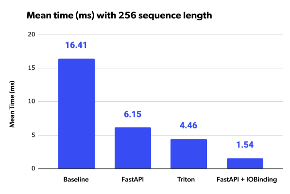
| 256 | 16.41 | 0.18 |
Deploy the Optimized Model on FastAPI
Here is the code for the FastAPI app that serves our optimized Question and Answer model:
Here are the results for the benchmark:
| Sequence Length | Mean Time (ms) | STD Time (ms) |
|---|---|---|
| 32 | 3.47 | 0.09 |
| 64 | 3.84 | 0.2 |
| 128 | 4.66 | 0.21 |
| 256 | 6.15 | 0.12 |
With just a few lines of code, we deployed an API that processes input and returns the output of the model in just a few milliseconds! Pretty cool, right?
| Sequence Length | Baseline | Opt. + FastAPI (ms) | Speed-up |
|---|---|---|---|
| 32 | 14.72 | 3.47 | x4.24 |
| 64 | 14.71 | 3.84 | x3.83 |
| 128 | 14.99 | 4.66 | x3.21 |
| 256 | 16.41 | 6.16 | x2.66 |
Using our optimized model and the ONNX Runtime, we can enjoy a nice speed-up of x2.6 for the longest sequence length! But now that we have already optimized the model, what else can we do to accelerate inference time even more? Let’s check it out!
Deploy the Optimized Model on Triton
Although FastAPI is a great tool and an enormous contribution to the open-source community, it wasn’t explicitly designed for deploying ML models. Its scope is much broader and, thus, lacks some functionalities that are much needed for deploying models: dynamic batching, auto-scaling, GPU management, model version control, and more.
If you are looking for these features, there’s another option. We are talking about NVIDIA’s inference server, Triton. Triton is an open-source solution for fast and scalable inferencing. With minimal effort, you can have your model deployed and enjoy the great features Triton has to offer!
All you need to get your model up and running in Triton is a simple configuration file specifying the inputs and outputs of the model, the chosen runtime, and the hardware resources needed. You can even leave the inputs and outputs unspecified, and Triton will try to detect them automatically from the model file! Here is the config file for our example:
We include some explanations of the variables and their values below:
max_batch_size: 0indicates that we don’t want to perform dynamic batching.- The
-1in the dimensions of the inputs and outputs means that those dimensions are dynamic and could change for each inference request. For example, if we receive a longer sequence, we could expect the second dimension ofinput_idsto be bigger. - The
instance_groupproperty lets us specify how many copies of our model we want to deploy (for load balancing) and which hardware they should use. Here we are just simply deploying one instance running on GPU.
Here is the benchmark for the optimized model deployed on Triton:
| Sequence Length | Mean Time (ms) | STD Time (ms) |
|---|---|---|
| 32 | 2.08 | 0.05 |
| 64 | 2.48 | 0.09 |
| 128 | 3.21 | 0.11 |
| 256 | 4.46 | 0.18 |
And here is the comparison with the baseline:
| Sequence Length | Baseline | Opt. + FastAPI (ms) | Speed-up |
|---|---|---|---|
| 32 | 14.72 | 2.08 | x7.07 |
| 64 | 14.71 | 2.84 | x5.93 |
| 128 | 14.99 | 3.21 | x4.66 |
| 256 | 16.41 | 4.46 | x3.67 |
As we can see, with little effort, Triton out-of-the-box achieves a speed-up of x3.67! Also, we didn’t have to code anything! Triton processes the inputs, calls the model, and returns the outputs all by itself, which will surely save you some time.
Although vanilla Triton achieved very good results, the tool has much more to offer than what we include in this blog post. Activating dynamic batching could save huge processing times by batching multiple requests, without significantly delaying response time. Model version management could help us test new versions of the model before taking them to production or allow us to have multiple versions of the model deployed simultaneously. Instance management enables us to perform load balancing or have multiple instances of the model for redundancy. With all these features and much more, Triton should definitely be amongst your first options for deploying models at scale!
Deploy the Optimized Model on FastAPI with IOBinding
We decreased inference time by a factor of 3.67. However, looking at the results of the benchmarks, you might have noticed something is off—the inference time appears to be increasing with the sequence length. This is due to poor management of GPU memory allocation and data transfer on our side. We will take one more step in optimizing inference time, applying a very cool technique called IOBinding.
IOBinding allows the user to copy the model's inputs to GPU (or other non-CPU devices) and allocate memory for the outputs on the target device without having to do so while running the computational graph of the model. This saves huge processing times during inference, especially if inputs and outputs are very large!
Here is the new code for the FastAPI app that serves our model, now with IOBinding activated.
Applying this optimization is not straightforward and requires a bit more code, but it sure is worth it. Check the results of the benchmark!
| Sequence Length | Mean Time (ms) | STD Time (ms) |
|---|---|---|
| 32 | 1.43 | 0.03 |
| 64 | 1.45 | 0.02 |
| 128 | 1.49 | 0.09 |
| 256 | 1.54 | 0.1 |
| Sequence Length | Baseline | Opt. + FastAPI (ms) | Speed-up |
|---|---|---|---|
| 32 | 14.72 | 1.43 | x10.29 |
| 64 | 14.71 | 1.45 | x10.14 |
| 128 | 14.99 | 1.49 | x10.06 |
| 256 | 16.41 | 1.54 | x10.65 |
FastAPI with IOBinding achieves almost constant execution time, even for higher sequence lengths! This allows us to achieve a x10 speed-up!

Closing Thoughts
Throughout this blog post, we saw various techniques for reducing the inference time and size of the model without losing much accuracy. We managed to decrease the model size by more than half its size and accelerate inference time by x7.73! We also presented two different tools for deploying your model and showed you how you can optimize serving in order to achieve a x10 speed-up!
Transformer models are the future. With the tools we just provided, you will be able to run state-of-the-art models much faster and with fewer resources, saving you time, effort and money.
Transformers in your next project
Are you having some concerns about it?

Wondering how AI
can help you?

Terms and Conditions | © 2026. All rights reserved.